kmerExtractor user manual

Below we present examples of how to use the main functions of the software.

Import libraries

[1]:

import pandas as pd
import matplotlib.pyplot as plt

# software to extract the k-mers
import kmerExtractor as kex

Compute k-mers

Specify the corresponding directory of the FASTA files from which you want to extract the k-mers, and the directory where you want to save the output files. Also define the window size (in base pairs) for which you want the frequency of k-mers to be counted.

In this case we will use the genome of arabidospsis, tomato and maize, with a window size of \(100000\) bp for all genomes.

[2]:

filepath_ara = '../input_data/arabidopsis_genome.fasta'
filepath_tom = '../input_data/tomato_genome.fasta'
filepath_mz = '../input_data/maize_genome.fasta'
output_path = '../output_data'
window_size = 100_000

Now use the kmers_by_window_opt function to calculate the k-mers of each genome for the \(k\) of your choice.

In the output file, the first column indicates the chromosome, the second column the window index, the third and fourth columns indicate the start and end position of the window respectively, and the rest of the \(4^k\) columns correspond to the k-mer frequencies. This data is saved in a csv file and stored in a dataframe for downstream analysis within the tutorial.

The resulting dataframe for arabidopsis 2-mers looks like shown below.

[3]:

df_2mers_ara = kex.kmers_by_window_opt(filepath_ara, k=2, window_size=window_size, output_path=output_path)
df_2mers_tom = kex.kmers_by_window_opt(filepath_tom, k=2, window_size=window_size, output_path=output_path)
df_2mers_mz  = kex.kmers_by_window_opt(filepath_mz,  k=2, window_size=window_size, output_path=output_path)
df_2mers_ara

100%|████████████████████████████████████████| 1537509/1537509 [00:45<00:00, 33733.02it/s]
100%|██████████████████████████████████████| 10090326/10090326 [04:45<00:00, 35388.84it/s]
100%|██████████████████████████████████████| 25502007/25502007 [12:31<00:00, 33940.82it/s]

[3]:

	chromosome	window	start	end	AA	AC	AG	AT	CA	CC	CG	CT	GA	GC	GG	GT	TA	TC	TG	TT
0	chr1	0	1	100000	11617	5201	5956	9480	6269	3277	2412	5588	6375	2998	3460	5248	7993	6069	6253	11803
1	chr1	1	100001	200000	10857	5241	5871	8727	6080	3516	2983	5895	6670	3174	3758	5578	7089	6544	6567	11449
2	chr1	2	200001	300000	10623	5144	6129	8658	6350	3575	2655	6386	6617	3378	3616	5325	6964	6869	6536	11174
3	chr1	3	300001	400000	9548	5117	6328	7979	6483	4297	2771	6834	6625	3923	4047	5310	6315	7049	6759	10614
4	chr1	4	400001	500000	11515	5294	5692	9068	6225	3578	2638	5896	6455	3027	3592	5271	7375	6438	6422	11513
...	...	...	...	...	...	...	...	...	...	...	...	...	...	...	...	...	...	...	...	...
1190	chr5	267	26700001	26800000	11432	5154	5970	9120	6440	3528	2620	5942	6521	3051	3289	5280	7283	6797	6262	11310
1191	chr5	268	26800001	26900000	11549	5299	5782	9116	6113	3457	2948	5881	6405	3068	3254	5222	7680	6575	5965	11685
1192	chr5	269	26900001	26975502	8826	4001	4609	6658	4719	2639	2158	4387	5163	2352	2573	3979	5386	4912	4726	8413
1193	chr5	269	26900001	26975502	8826	4001	4609	6658	4719	2639	2158	4387	5163	2352	2573	3979	5386	4913	4726	8413
1194	chr5	269	26900001	26975502	8826	4001	4609	6658	4719	2639	2158	4387	5163	2352	2573	3979	5386	4914	4726	8413

1195 rows × 20 columns

However, a most natural approach is to use \(k=3\), since the 3-mers represent codons, which encode for amino acids or signal the termination of protein synthesis (stop signals).

The resulting dataframe for arabidopsis 3-mers looks like below.

[4]:

df_3mers_ara = kex.kmers_by_window_opt(filepath_ara,k=3,window_size=window_size,output_path=output_path)
df_3mers_tom = kex.kmers_by_window_opt(filepath_tom,k=3,window_size=window_size,output_path=output_path)
df_3mers_mz = kex.kmers_by_window_opt(filepath_mz,k=3,window_size=window_size,output_path=output_path)
df_3mers_ara

100%|████████████████████████████████████████| 1537509/1537509 [00:54<00:00, 28160.74it/s]
100%|██████████████████████████████████████| 10090326/10090326 [05:59<00:00, 28039.88it/s]
100%|██████████████████████████████████████| 25502007/25502007 [15:53<00:00, 26741.24it/s]

[4]:

	chromosome	window	start	end	AAA	AAC	AAG	AAT	ACA	ACC	...	TCG	TCT	TGA	TGC	TGG	TGT	TTA	TTC	TTG	TTT
0	chr1	0	1	100000	4415	1966	2228	3008	1926	1096	...	776	2200	2016	1007	1349	1881	2682	2169	2422	4530
1	chr1	1	100001	200000	4026	1914	2114	2803	1849	1063	...	959	2339	2102	957	1432	2076	2324	2283	2489	4353
2	chr1	2	200001	300000	3899	1875	2138	2711	1863	1066	...	932	2572	2098	1085	1390	1963	2255	2477	2322	4120
3	chr1	3	300001	400000	3335	1760	2117	2336	1729	1110	...	833	2586	2041	1313	1456	1949	1998	2398	2334	3884
4	chr1	4	400001	500000	4629	1874	2085	2926	1929	1075	...	885	2301	2109	988	1406	1919	2499	2241	2414	4359
...	...	...	...	...	...	...	...	...	...	...	...	...	...	...	...	...	...	...	...	...	...
1190	chr5	267	26700001	26800000	4301	2000	2180	2951	1818	1114	...	891	2453	2014	1028	1297	1922	2394	2385	2340	4191
1191	chr5	268	26800001	26900000	4423	1999	2061	3066	1835	1072	...	973	2304	1962	937	1221	1845	2695	2302	2196	4492
1192	chr5	269	26900001	26975502	3366	1522	1803	2135	1467	797	...	704	1734	1585	738	960	1443	1861	1717	1716	3119
1193	chr5	269	26900001	26975502	3366	1522	1803	2135	1467	797	...	704	1734	1585	738	960	1443	1861	1717	1716	3119
1194	chr5	269	26900001	26975502	3366	1522	1803	2135	1467	797	...	704	1734	1585	738	960	1443	1861	1717	1716	3119

1195 rows × 68 columns

Read k-mer files if already computed

Calculating k-mers can take longer for larger genomes. That’s why you also have the option to load previously saved files, so you don’t have to recalculate the k-mers every time you want to plot some figures or do further analysis.

[5]:

df_2mers_ara = pd.read_csv(output_path +'/CGRW_k2_arabidopsis_genome.csv')
df_2mers_tom = pd.read_csv(output_path +'/CGRW_k2_tomato_genome.csv')
df_2mers_mz = pd.read_csv(output_path +'/CGRW_k2_maize_genome.csv')

df_3mers_ara = pd.read_csv(output_path +'/CGRW_k3_arabidopsis_genome.csv')
df_3mers_tom = pd.read_csv(output_path +'/CGRW_k3_tomato_genome.csv')
df_3mers_mz = pd.read_csv(output_path +'/CGRW_k3_maize_genome.csv')

Group all windows within each chromosome

If you don’t want the k-mer frequencies by windows within the chromosomes, you can get the cumulative frequencies for each chromosome as shown in the cell below. For example, the resulting dataframe for arabidopsis would have only 5 rows corresponding to its 5 chromosomes.

[6]:

df_2mers_ara_bychr = df_2mers_ara.groupby('chromosome').agg({k:'sum' for k in df_2mers_ara.columns[4:]})
df_2mers_tom_bychr = df_2mers_tom.groupby('chromosome').agg({k:'sum' for k in df_2mers_tom.columns[4:]})
df_2mers_mz_bychr = df_2mers_mz.groupby('chromosome').agg({k:'sum' for k in df_2mers_mz.columns[4:]})
df_2mers_ara_bychr

[6]:

	AA	AC	AG	AT	CA	CC	CG	CT	GA	GC	GG	GT	TA	TC	TG	TT
chromosome
chr1	3519572	1588202	1794811	2806911	1923811	1016038	697362	1798090	1930160	902322	1008839	1579754	2335983	1928721	1920061	3512205
chr2	2291405	1029105	1160640	1834416	1246754	672290	457569	1166315	1249456	584680	660355	1026228	1527955	1256858	1242154	2289303
chr3	2697289	1228414	1405644	2153303	1498561	804334	559027	1396347	1516501	714668	805341	1226134	1772296	1510857	1492635	2672182
chr4	2143926	980389	1109010	1707158	1184064	637226	439583	1110444	1195069	560350	630128	970513	1417419	1193357	1177332	2125863
chr5	3140913	1410681	1608073	2510382	1712226	907201	634608	1605965	1741333	808346	914520	1422652	2075592	1733770	1729636	3160014

Group all chromosomes

Furthermore, you can pool the k-mer frequencies of all the chromosomes and have the cumulative counts of the entire sequence.

[7]:

df_2mers_all = pd.DataFrame()
df_2mers_all['arabidopsis'] = df_2mers_ara_bychr.sum()
df_2mers_all['tomato'] = df_2mers_tom_bychr.sum()
df_2mers_all['maize'] = df_2mers_mz_bychr.sum()
df_2mers_all.T

[7]:

	AA	AC	AG	AT	CA	CC	CG	CT	GA	GC	GG	GT	TA	TC	TG	TT
arabidopsis	13793105	6236791	7078178	11012170	7565416	4037089	2788149	7077161	7632519	3570366	4019183	6225281	9129245	7623563	7561818	13759567
tomato	85677817	37700236	41002572	75901364	45946447	25138712	11804902	40969026	42920385	18121904	25183170	37739813	65737185	42898271	45974544	85737480
maize	161563751	108257047	128688710	136989307	133796230	120957040	87977339	128781627	129723428	112442579	121098322	108465666	110415392	129855155	133966157	161938131

k-mer figures

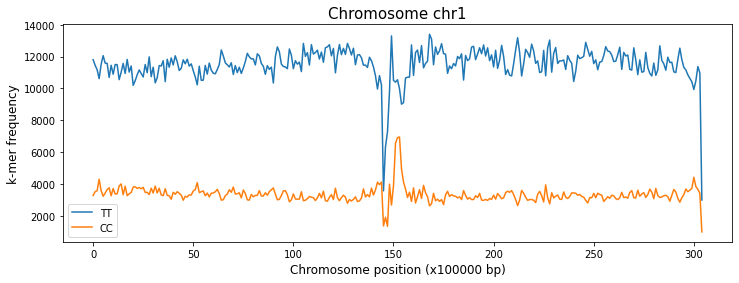
Plot k-mers across windows

With the plot_kmers_across_windows function you can plot the frequencies of the k-mers of your choice across the windows of a specified chromosome.

[8]:

a = kex.plot_kmers_across_windows(df_2mers_ara,['TT','CC'],'chr1')

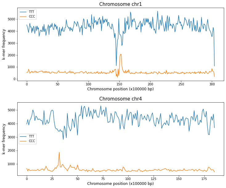
You can also use this function to compare, placing the plot of different chromosomes on different axes within the same figure.

[9]:

fig,ax = plt.subplots(2,1,figsize=(12,10),gridspec_kw={'hspace': 0.3})

kex.plot_kmers_across_windows(df_3mers_ara,['TTT','CCC'],'chr1',ax=ax[0])
kex.plot_kmers_across_windows(df_3mers_ara,['TTT','CCC'],'chr4',ax=ax[1])

plt.show()

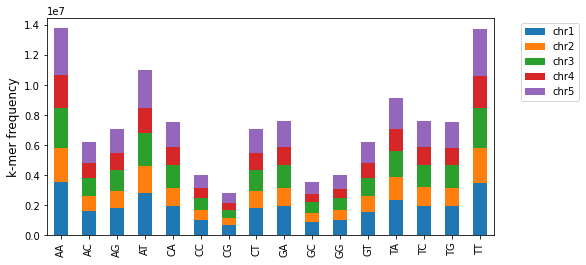
Plot k-mer frequencies within each chromosome

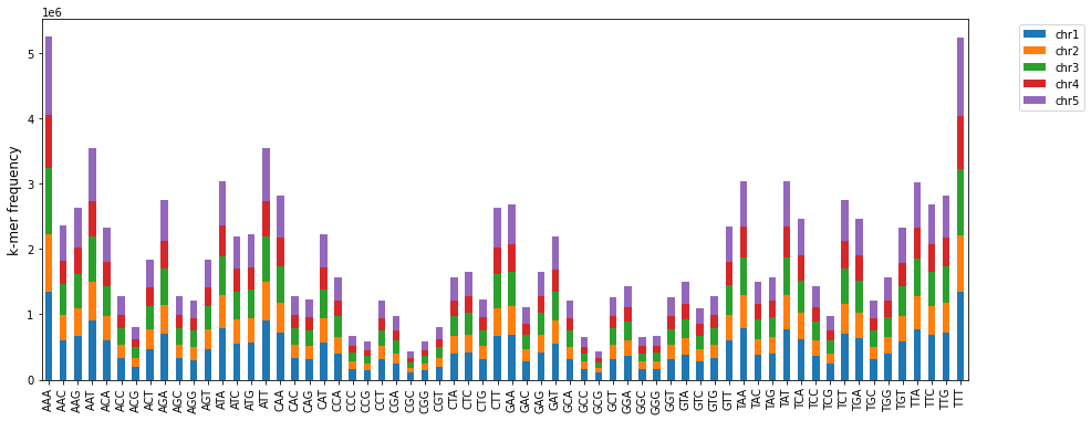
The plot_kmers_freq_within_chromosomes function makes a stacked bar graph of the frequency of different k-mers per chromosome. For the same k-mer, each stacked bar represents a different chromosome of the corresponding color.

[10]:

b = kex.plot_kmers_freq_within_chromosomes(df_2mers_ara,figsize=(8,4))

[11]:

c = kex.plot_kmers_freq_within_chromosomes(df_3mers_ara)

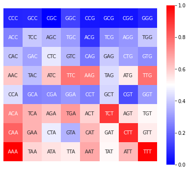
Plot FCGR structure

The technique to show the k-mer frequencies as images is known as Frequency Chaos Game Representation (FCGR). It corresponds to a matrix of dimensions \(2^k \times 2^k\); with the upper left corner equal to the k-mer of C, the upper right corner the k-mer of G, the lower left corner the k-mer of A, and the lower right corner the k-mer of T.

The plot_FCGR function plots the FCGR of a sequence as a heatmap that allows to appreciate the relative frequencies of each k-mer. You can plot the FCGR for a specific chromosome and window, the cumulative frequency for an entire chromosome (if no window is specified), or the cumulative frequency for the entire genome (if neither chromosome nor window is specified).

[12]:

d = kex.plot_FCGR(df_3mers_ara,'chr1',window=145)

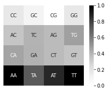
You can also adjust the size of the figure and the colormap to your preference as shown below

[13]:

e = kex.plot_FCGR(df_2mers_tom,'chr6',figsize=(4,3),colormap='Greys')

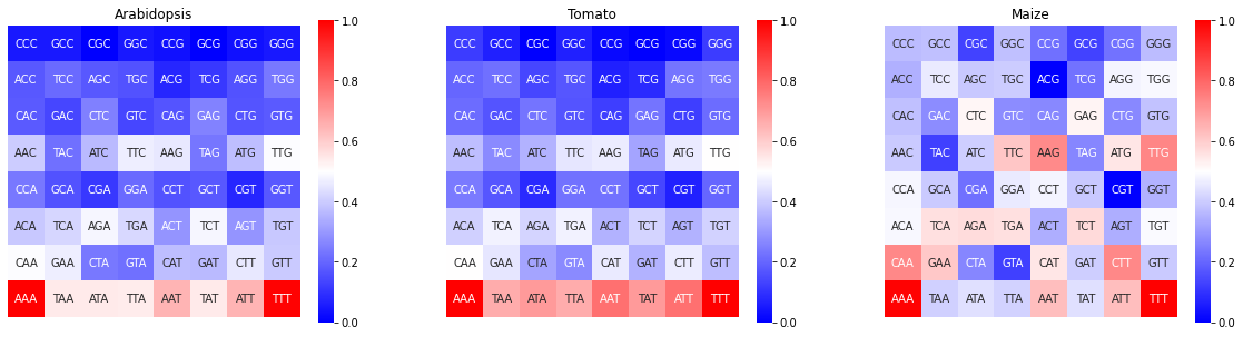
Aditionally, is possible compare the FCGR of multiple genomes as shown in the following cell

[14]:

fig,ax = plt.subplots(1,3,figsize=(20,5))

kex.plot_FCGR(df_3mers_ara,ax=ax[0])
kex.plot_FCGR(df_3mers_tom,ax=ax[1])
kex.plot_FCGR(df_3mers_mz,ax=ax[2])

ax[0].set_title('Arabidopsis')
ax[1].set_title('Tomato')
ax[2].set_title('Maize')

plt.show()

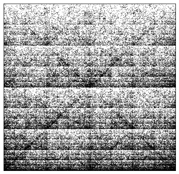
Plot CGR

Finally, although it is not the main objective of the software, a function to generate the CGR image of a sequence is included. In the following example, the FASTA file of the Arabidopsis genome is read and the CGR of the first 100 kb is generated.

[15]:

import re

# Read FASTA file with complete genome separated by chromosomes
f_in = open(filepath_ara, 'r')
all_file = f_in.read()
f_in.close()

# join lines
seq_all = "".join(all_file.split("\n"))
del all_file

# Split sequence by chromosomes
seq_bychr = re.split('>chr[1-9]*', seq_all)[1:]
del seq_all

# plot CGR of the first chromosome, first window (first 100 Kb)
f = kex.plot_CGR(seq_bychr[0][:100_000],markersize=0.2)

100%|████████████████████████████████████████| 100000/100000 [00:00<00:00, 1886046.78it/s]